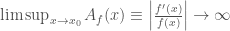
This last semester, I ran a fun, informal master class in problem solving. Actually, a graduate student of mine — Yunfeng Hu — who is an expert problem solver, produced all the problems from the immense library he built up over his undergraduate career in China.
I believe that the art and culture of problem solving is not as widely valued in the USA as it ought to be. Of course there are those that do pursue this obsession and we end up with people with high scores on the Olympiad and Putnam competitions. But many (most?) do not develop this skill to any great degree. While one can certainly argue that too much emphasis on problem solving along the lines of these well known competitions does not help very much in making real progress in current research, I would argue that many have fallen off the other side of the horse — many are sometimes hampered by their lack of experience in solving these simpler problems.
Here is a problem that arose in our Wednesday night session:
Suppose that
 (1)
(1)
for all  , that
  is continuous and differentiable, and that
  .
.
Prove that  everywhere.
Perhaps you want to fiddle with this problem before looking at some solutions. If so, wait to read further.
Here are three solutions: in these first three solutions we are dealing with  and so we will denote
  by
by  .
.
(Solution 1) Consider all the solutions to  and
and  . These are all curves in
  of the form
  and
and  We note that if
  is any function that satisfies equation (1), then everywhere its graph intersects a graph of a curve of the form for some
  , the graph of
  must cross the graph of
  if we are moving form left to right the graph of moves from above to below the graph of
  . Likewise, crosses any
  from below to above, when moving from left to right in
  . Now, supposing that
  at some
  . Then simply choose the curves
  and
and  as fences that cannot be crossed by
  (one for
  and the other for
  to conclude that can never equal zero. (Exercise: Verify that this last statement is correct. Also note that assuming is enough since, if instead
  then
then  also satisfies (1) and is positive at )
(Solution 2) This next solution is a sort of barehanded version of the first solution. We note that equation (1) is equivalent to
 (2)
(2)
and if we assume that  on
on  , then this of course turns into
 . (3)
. (3)
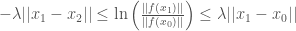
Assume that ![[x_0,x_1]\in E](https://s0.wp.com/latex.php?latex=%5Bx_0%2Cx_1%5D%5Cin+E&bg=ffffff&fg=444444&s=0&c=20201002) and divide by to get
and divide by to get  Integrating this, we have
  or
or
 (4)
(4)
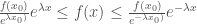
Now assume that . Define  and
and  Note that
  implies that
  and
and  implies that
  Use equation (4) together with
  or
or  , to get a contradiction if either or
(Solution 3) In this approach, we use the mean value theorem to get what we want. Suppose that  . We will prove that
  on the interval
 ![I = [x_0 - \frac{1}{2\lambda}, x_0 + \frac{1}{2\lambda}]](https://s0.wp.com/latex.php?latex=I+%3D+%5Bx_0+-+%5Cfrac%7B1%7D%7B2%5Clambda%7D%2C+x_0+%2B+%5Cfrac%7B1%7D%7B2%5Clambda%7D%5D&bg=ffffff&fg=444444&s=0&c=20201002) .
.
(exercise) Prove that this shows that 

 . (Of course, all this assumes Equation (1) is true.)
Assume that  . Then the mean value theorem says that
 (5)
(5)
for some  . But using equation (1) and the fact that , this turns into
  By the same reasoning, we get that
  for some
  , and we can conclude that
  . Repeating this argument, we have
 (6)
(6)
for some  , for any positive integer
  . Because is continuous, we know that there is an
  such that
  . Using this fact together with Equation (6), we get
 (7)
(7)
which of course implies that
Now we could stop there, with three different solutions to the problem, but there is more we can find from where are now.
Notice that one way of looking at the result we have shown is that if
(1) is differentiable,
(2)  and
and
(3) for some  , we have that
  when
when  and
and ![x\in [x_0 - \delta, x_0 + \delta]](https://s0.wp.com/latex.php?latex=x%5Cin+%5Bx_0+-+%5Cdelta%2C+x_0+%2B+%5Cdelta%5D&bg=ffffff&fg=444444&s=0&c=20201002) ,
,
then
 (8)
(8)
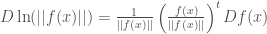
Note also that if we define
 (9)
(9)
we find that
 (10)
(10)
Let  denote the continuously differentiable functions from
  If we define
  we find that not only is
  not all of , we also have functions satisfying
 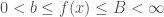 whose
whose  . So we will restrict the class of functions a bit more. The space of continuously differentiable functions from
  to
to  ,
,  , where
 ![K = [-R,R]](https://s0.wp.com/latex.php?latex=K+%3D+%5B-R%2CR%5D&bg=ffffff&fg=444444&s=0&c=20201002) (compact!), is closer to what we want. Now,
(compact!), is closer to what we want. Now,  contains only those functions which have a root in
  .
.
We will call the functions in  functions with maximal growth rate
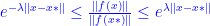
  . This is a natural moduli for functions when we are studying stuff whose (maximal) grow rate depends linearly on the current amount of stuff. Of course populations of living things fall in the class of things for which this is true. from the proofs above, we know that if
  , then it’s graph lives in the cone defined by exponentials. More precisely
If  then for
  ,
,  and for
  we have
(Exercise) Prove this. Hint: use the first proof where instead of  you use
  and let
  .
.
(Remark) Notice that Equation (10) and  implies that scaling a function in
  by any non-zero scalar yields another function in
  As a result, we might choose to consider only

or

In both cases we end up with subsets that generate when we take all multiples of those functions by nonzero real numbers.
(Exercise) If we move to high dimensional domains, how wild can the compact set be and still get these results? It must clearly be connected, so in  we are already completely general with our above.
Moving back to Equation (1), we can look for generalizations: for example, will this result hold when  How about when maps from one Banach space to another? How about the case in which is merely Lipschitz?
Lets begin with 
In this case, the appropriate version of Equation (1) is
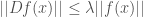 (11)
(11)
where  denotes the operator norm of the derivative
  and
and  is the euclidean norm of in
Notice that
 (12)
(12)
where  is an
is an  dimensional row vector and is an
  dimensional matrix. (Thus the gradient vector is the transpose of the resulting dimensional row vector.) Now we can use this to get the result.
Let  be the arclength parameterized line segment that starts at
  and ends at
  the The above equation tells us that
 (13)
(13)
Thus, we can conclude that

which implies that
and we can proceed as we did in the second proof of the problem in the case that  We end up with the following result
If  and
and  , then
for all 
(Exercise) Show that this result implies that if f(x) = 0 anywhere, it equals 0 everywhere.
(Exercise) Show that this is implies the one dimensional result we proved above (the first theorem we proved above).
(Exercise) Our proof of the result for the case  can be carried over to the case of
  where
where  are Banach Spaces — carry out those steps!
We come now to the question of what we can say when we are less restrictive with the constraints on differentiability. We consider the case in which is Lipschitz. The complication here is that while we know that is differentiable almost everywhere, it might not be differentiable anywhere on the line segment from to .
Consider a cylinder  , with radius
  and axis equal to the segment from
  Let
Let  . Since is differentiable almost everywhere, we have that
  . Therefore almost every segment
  generated by the intersection of a line parallel to the cylinder axis and the cylinder, intersects
  in a set of length
  . We can therefore choose a sequence of such segments converging to
 ![[x_0,x_1].](https://s0.wp.com/latex.php?latex=%5Bx_0%2Cx_1%5D.&bg=ffffff&fg=444444&s=0&c=20201002)

Since  exists
  almost everywhere on the segments
 ![[x_0^k, x_1^k]](https://s0.wp.com/latex.php?latex=%5Bx_0%5Ek%2C+x_1%5Ek%5D&bg=ffffff&fg=444444&s=0&c=20201002) and is continuous everywhere, we can integrate the derivatives to get:
and is continuous everywhere, we can integrate the derivatives to get:
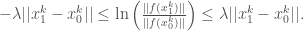
And because is continuous we get that

so that we end up with the same result that we had for differentiable functions.
There are other directions to take this.
From the perspective of geometric objects, the ratio  is a bit funky — for example, if
  volume of a set
  , where can be thought of as the center of the set, we have that will be a vectorfield
  times
times  restricted to the
  . Thus,
  will be an
  -dimensional quantity and a -dimensional quantity. We would usually expect there to be exponents, as in the case of the Poincare ineqaulity, making the ratio non-dimensional.
On the other hand, one can see this ratio as a sort of measure of reciprocal length of the objects we are dealing with. From the perspective, this result seems to say that no matter what you do, you cannot get to objects with no volume from objects with non-zero volume without getting small (i.e. without the reciprocal length diverging). This is not profound. On the other hand, that ratio is precisely what is important for certain physical/biolgical processes. So this quantity being bounded has consequences in those contexts.
This does not lead to a new theorem: as long as the set evolution is smooth, the and are just a special case where  and even though actually computing everything from the geometric perspective can be interesting, the result stays the same.
in order to move into truly new territory, we need to consider alternative definitions, other measures of change, other types of spaces. An example might be the following:
Suppose that  is a metric space and
  . Suppose that
  is continuous and is a geodesic in the sense that for any three points in ,
  , we have that
If:
(1) for any two points in the metric space there is a gamma containing both points and
(2) for all such  ,
,  is differentiable
(3) and 
then, we have that
 (14)
(14)
And, again we get the same type of result for this case as we got in the Euclidean cases above.
(Exercise) Prove Equation (14).
(Remark) We start with any metric space and consider curves ![\gamma:[a,b]\subset\Bbb{R}\rightarrow X](https://s0.wp.com/latex.php?latex=%5Cgamma%3A%5Ba%2Cb%5D%5Csubset%5CBbb%7BR%7D%5Crightarrow+X&bg=ffffff&fg=444444&s=0&c=20201002) for which
for which
 .
.
We call such curves rectifiable. We can always reparameterize such curves by arclength, so that ![\gamma(s) = \gamma(s(t)), t\in[0,l(\gamma)]](https://s0.wp.com/latex.php?latex=%5Cgamma%28s%29+%3D+%5Cgamma%28s%28t%29%29%2C+t%5Cin%5B0%2Cl%28%5Cgamma%29%5D&bg=ffffff&fg=444444&s=0&c=20201002) and
and ![l([\gamma(s(d)),\gamma(s(c))] ) = d-c](https://s0.wp.com/latex.php?latex=l%28%5B%5Cgamma%28s%28d%29%29%2C%5Cgamma%28s%28c%29%29%5D+%29+%3D+d-c&bg=ffffff&fg=444444&s=0&c=20201002) . We will assume that all curves have been reparameterized by arclength. Now define a new metric
. We will assume that all curves have been reparameterized by arclength. Now define a new metric

You can check that this will not change the length of any curve. Define an upper gradient of be any non-negative function  such that
  .
.
Now, if  , we again get the same sort of bounds that we got in equation (14) if we replace
  with
with  . To read more about upper gradients, see Juha Heinonen’s book Lectures on Analysis in Metric Spaces.
While there are other directions we could push, what we have looked at so far demonstrates that productive exploration can start from almost anywhere. While we encounter no big surprises in this exploration, the exercise illuminates exactly why the result is what it is and this solidifies that understanding in our minds.
Generalization is not an empty exercise — it allows us to probe the exact meaning of a result. And that insight facilitates a more robust, more useful grasp of the result. While some get lost in their explorations and would benefit from touching down to the earth more often, it seems to me that in this day and age of no time to think, we most often suffer from the opposite problem of never taking the time to explore and observe and see where something can take us.

 and
and  Boundaries
  functional was actually computing the flat norm for boundaries, we suggested this gave us a computational route to statistics in spaces of shapes. While earlier work certainly touched on this idea of using the flat norm for inference in shape spaces — see
  , this becomes

 .
. . This is illustrated in the first figure.
 , the optimal linear approximation to f at a, is another, very useful way to think about the derivative. Here, we focus on the fact that the tangent line at
  ,
, ,
, ,
,  as
as  , and the tangent line L is the graph of the function
  .
. have the form
  ,
,  a scalar, and (2)
  as
as ![\left|f(x) - (f(a) + \hat{L}_a(x-a))\right| \leq (\sup_{|s|\in[0,\epsilon]} |g(s)|)|h|](https://s0.wp.com/latex.php?latex=%5Cleft%7Cf%28x%29+-+%28f%28a%29+%2B+%5Chat%7BL%7D_a%28x-a%29%29%5Cright%7C+%5Cleq+%28%5Csup_%7B%7Cs%7C%5Cin%5B0%2C%5Cepsilon%5D%7D+%7Cg%28s%29%7C%29%7Ch%7C&bg=ffffff&fg=444444&s=0&c=20201002) for
for ![h\in[-\epsilon,\epsilon]](https://s0.wp.com/latex.php?latex=h%5Cin%5B-%5Cepsilon%2C%5Cepsilon%5D&bg=ffffff&fg=444444&s=0&c=20201002) ,
,
 -balls centered on
  -ball, the graph stays in the wider cone, while in the smaller,
  -ball the graph stays in the narrower cone.
 ,
, to be the ball of radius
  ,
, ,
, to be the smallest closed cone, symmetrically centered on
  , and
, and to be the angular width of

 } using the facts that (1) the above inequality defines cones that are almost symmetric about
 ![(x-a,y-f(a)) \in [-\epsilon,\epsilon] \times(-\infty,\infty)](https://s0.wp.com/latex.php?latex=%28x-a%2Cy-f%28a%29%29+%5Cin+%5B-%5Cepsilon%2C%5Cepsilon%5D+%5Ctimes%28-%5Cinfty%2C%5Cinfty%29&bg=ffffff&fg=444444&s=0&c=20201002)
 can have any dimension from 1 to n. For nicely behaved k-dimensional sets, the tangent cone will also be k-dimensional. In the case of the usual derivative of functions from
  with 1-dimensional sets. Moving to tangent cones, we can approximate one dimensional sets which are not graphs or, more generally, arbitrary subsets of
  at
at  by
by  . (This moves
  . Use a projection center at 0 to project the translated
  onto the sphere of radius
  . That is,


 ‘s going to zero;
  will do. Thus the tangent cone of
  is given by:

 , the k-dimensional density of F at p.
 such that it agrees with the volume of the unit ball in
  when k is an integer (there is a standard way to do this using
  functions). Let
  measure k-dimensional volume. Typically this will be k-dimensional Hausdorff measure,
  . Whatever intuitive idea you have of k-dimensional measure is good enough for our purposes. (At the end of this post I also define Hausdorff measures more carefully.)

 and
and  respectively.

 , converges weakly to
 .
. while the dashed green line indicates the boundary of the support of

 :
: , where
  . Here,
  is the diameter of
  .
.
 where the infimum is taken over all covers whose elements with maximal diameter d.
 , there is a cover
  of
of  , such that
  . Then for
  ,
,  .
.
 . And by use of mappings, this can take us quite a ways in computing
  for integral k and rather general
  then
then  and
and  for
for  .
.
You must be logged in to post a comment.